The Race
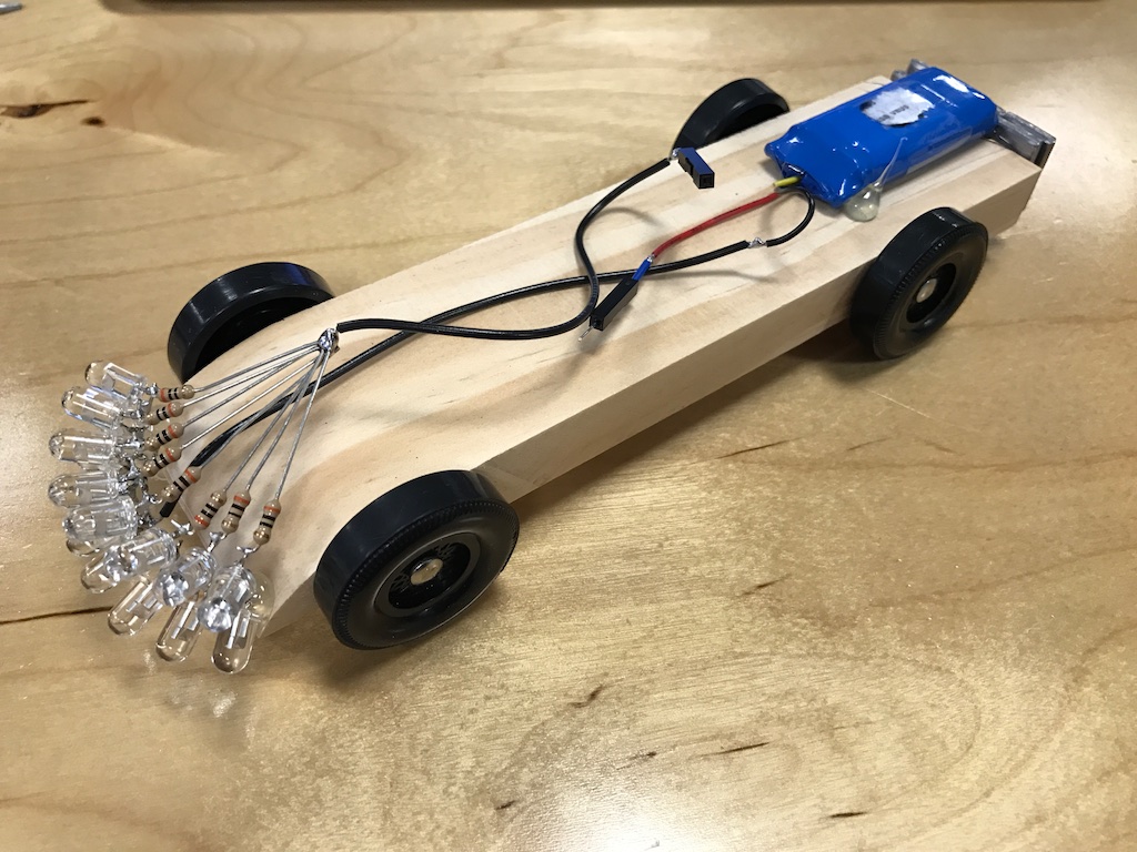
With no sweet hoverboard to race, I decided to temporarily shelve the physics and quickly slap something else together. With a battery and a boatload of infrared LEDs, I came up with this:
See, I knew that the track uses an infrared beam-break sensor to detect when a car passes the finish line. A beam break has a light source hitting a sensor and then detects when an object blocks the light and casts a shadow on the sensor. My hope was that with enough IR light, I could fill in the shadow of any car in front of me and prevent it from being detected by the beam-break.
This would prevent the system from recognizing that they finished in front of me and make me win by default BWAHAHAH!
The LEDs drew a pretty decent 124mA of current: 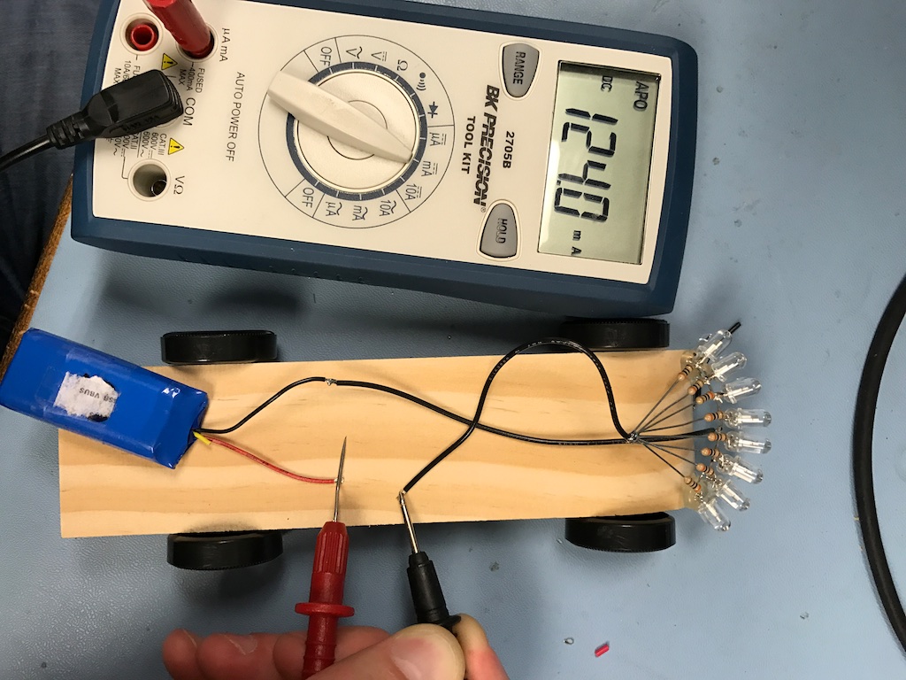
And were pretty bright in the infrared spectrum as shown by this IR image taken with a special camera from our lab:
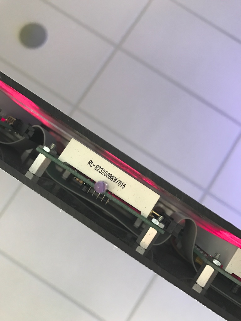
Sadly, this last-minute strategy didn’t pan out. The sensors weren’t fooled in any of the races. Some pre-race reconnaissance showed that I was right about the infrared beam-break at the finish line:
But the detector was on the bottom of the track and down a deep hole that would prevent indirect light from my car from having a major impact:
I asked the owner of the track if the IR light was modulated and he just laughed.
But hey, looks like I got 6th place anyway, fair and square!
Post race postulation
Though the race had come and gone, I wasn’t content to give up that easily on the concept of a hoverboard pinewood derby car. I really thought it was a cool idea and had been sitting on it for over a year. If I was going to give up on it, I decided that it would be because I deemed it to be impossible and not because I simply didn’t know how to do it. This whole thing was a crapshoot from the start, so I wasn’t going to be upset if it just turned out to be a really bad idea.
Besides, some of my worst ideas make the best blog posts.
Math
Though I had iterated on the design dozens of times in the real world, if I really wanted to optimize it, I was going to need a good mathematical model for what exactly was happening. This would require a formula to specify the magnetic field generated in the coil as well as a formula for how much current is induced in the metal plate. I was specifically curious if there was some tuning to be done that depended on the dimensions of the aluminum.
Mathematical models representing physical systems can get very complicated very quickly, so it’s best to simplify the system as much as possible. Rather than a rectangular or oval shaped coil, I decided to model a circular coil. More symmetry normally means easier math.
Indeed, I found a pretty simple formula for the magnetic field inside a current loop:
![]()
Unfortunately, this only indicates the magnetic field in the very center of the coil. Since my coil would be floating above my metal plate, I was going to need the formula for the magnetic field slightly below it:
Farther down on the same page, I found the formula for the magnetic field anywhere along the axis of a current loop where z represents how far you are away from the plane of the loop:
![]()
Easy, right?
Sadly, this only gives you the magnetic field along the exact axis of the coil. As soon as you move anywhere off that axis, things get very, very complicated. See, these formulae are simplified since you’re able to use the symmetry of the problem to cancel out a lot of complicated math.
This wouldn’t work for me though as I needed to know the magnetic field all along the aluminum plate in order to start calculating the force the coil generates.
Once you move off that exact axis, you need to take into account the impact of the current along every point in the coil while the direction of the current and its distance from your point changes as you move around the coil. This is the kind or problem that calculus was designed to solve, but even still, it would require a very, very complicated formula.
Even just determining the inductance of a coil of wire can be hard:
and involves somewhat arbitrarily defined variables like Y and O which have something to do with the skin effect at high frequencies.
I looked through some old textbooks for guidance, but I realized that even if I was able to determine the exact direction and magnitude of the magnetic field along the aluminum plate, I still wasn’t quite certain how to model the induced current in the plate and ultimately the force generated.
This is where computer models become super useful.
Simulation
Alright, let’s try this “MaxFEM” thing out…
Oh sweet!
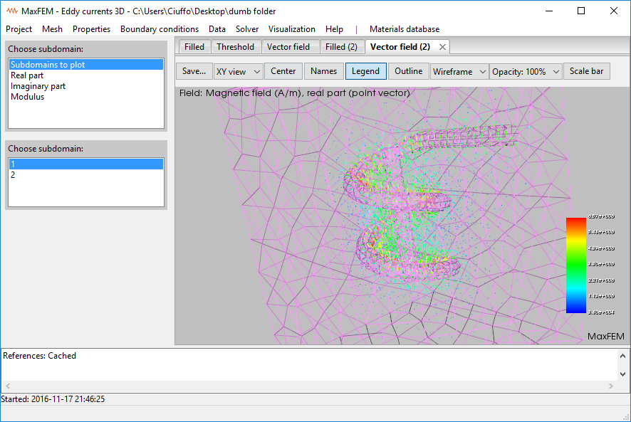
MaxFEM is a software package that can simulate several different types of 2D and 3D problems. It took a little bit of work to get it to run though. Here are my notes on the matter:
Installed Python 2.7 64 bit for Windows.
Modified wx_version to accept version 3.0 instead of 2.4
modified PanelVisual.py to add ex.locale=wx.Locale(wx.LANGUAGE_ENGLISH)
Install VTK
Add crap to PYTHONPATH export PYTHONPATH=/home/doriad/bin/VTK/lib:/home/doriad/bin/VTK/lib/site-packages:/home/doriad/bin/VTK/Wrapping/Python:$PYTHONPATH
With these changes, MaxFEM will run successfully. The software is pretty neat to play with. The help file is useful and walks you through the myriad different pre-built simulations that come with the software.
What I found is that creating your own simulations is very, very difficult.
I gave up on 3D simulations pretty early. Since my system is mostly symmetrical, I figured I could get by with their “Eddy currents axisymmetric” simulator. To make simulations, you first need to create “meshes.” These split the simulation space into discrete cells that make the math much simpler for the computer.
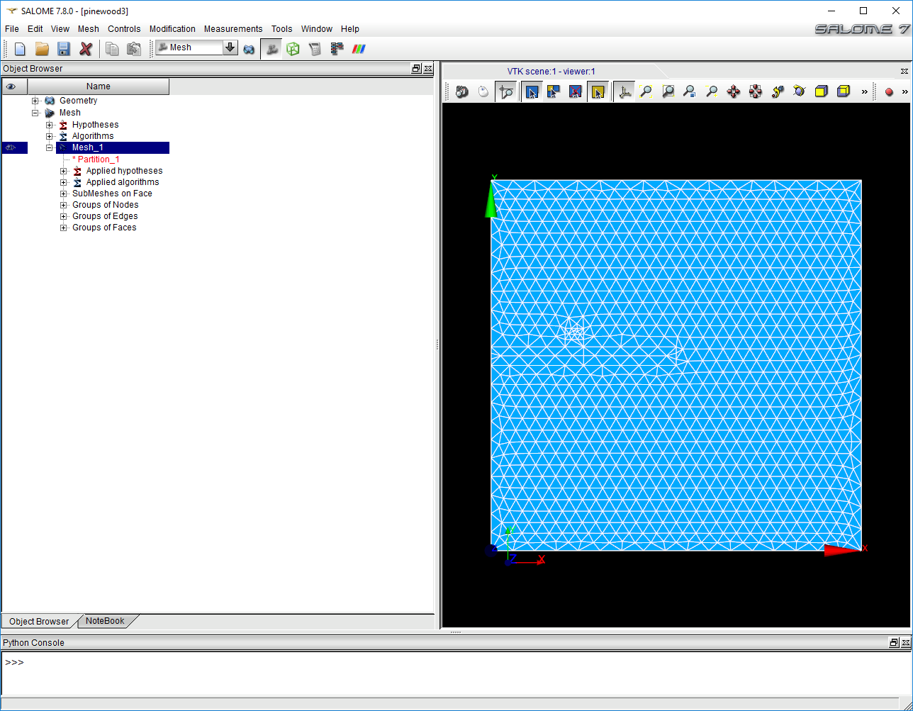
Generating meshes is a bit of an art. The makers of MaxFEM recommend using Salome for generating meshes. After a lot of tinkering, I was able to create this mesh that illustrates a radial cross section of a donut floating over a plate of aluminum:
Unfortunately, I was never able to get this mesh to work in MaxFEM. After exporting my Mesh_1 as a .unv file, MaxFEM would let me use it and even begin simulating, but somewhere in that simulation, the software would catch and error and halt before it finished producing the data.
I’ve included the .hdf Salome project file at the end of this article. You’re welcome to try getting it to work.
Simulation (again)
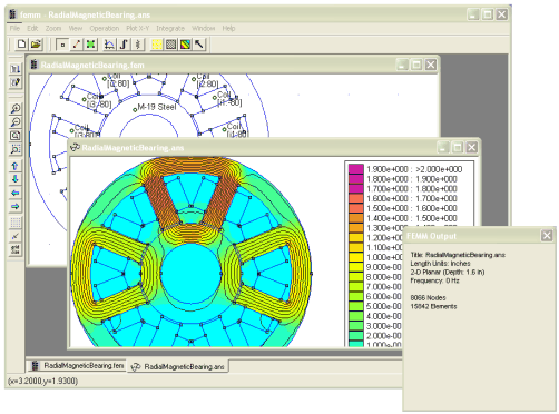
Rather than clicking the first google result, this time around I went a little down the page and found FEMM:
I can’t speak to whether it’s better or worse than MaxFEM (it doesn’t have any 3D simulation tools), but it does perform its own mesh generation which takes that major stumbling block away.
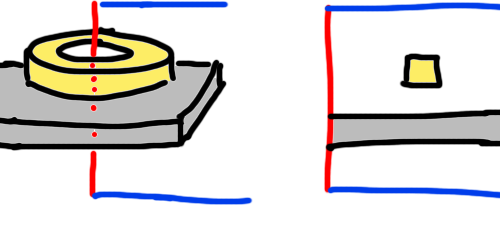
FEMM also has support for Axisymmetric simulation. Using this problem type, I broke my simulation down like this:
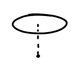
FEMM lets you treat blocks as coils of magnet wire. Cutting a cross-sectional slice out of this setup starting from the center axis yields the drawing on the right. This is what I needed to recreate in FEMM.
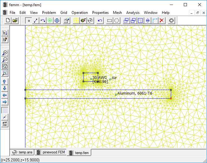
There are tons of tutorials online on how to use FEMM, so if you want to know exactly what I did, you can consult those. The end result was this:
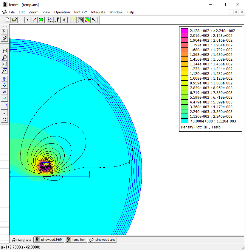
In the above example, I configured the coil to have a radius of 22mm and 96 turns and be driven with three amps of AC current at 2kHz. My actual circuit was driving with a square wave instead of sinusoidal AC, but I figured it was close enough since a pretty substantial portion of the energy in a square wave is in its fundamental frequency sinusoidal component. After running the analysis, I took a look at the results and turned on heat map for magnetic flux density:
PREEEETYYYY
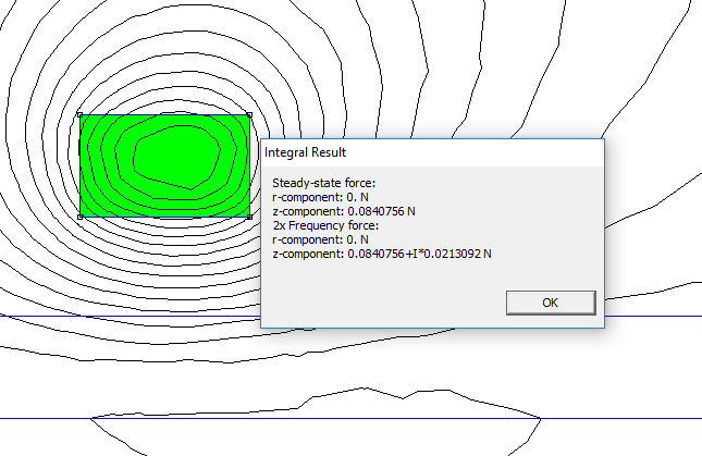
Now to get down to some science. I needed to figure out exactly how much upward force my coil generated. For this, I used the “block integral” function which is able to compute certain quantities by integrating over a whole shape. In this case I selected the cross section of my wire coil and selected “Lorentz Force.”
There’s a bit of math needed to explain why there is a steady-state force and 2X frequency force. The short story is that the force is related to the square of the magnetic flux density and our magnetic flux density (and our current) go as
![]()
. There’s a neat mathematical identity that shows that
![]()
. This leaves you with a steady-state component and a component that oscillates at 2X the input frequency with some amount of phase shift indicated by the complex number notation.
This doesn’t matter a whole lot for us though. For the most part the steady-state force and the magnitude of the 2X frequency force respond the same way to changes in the problem setup, and our goal here is to just maximize them as much as possible. For the rest of this problem, I focused exclusively on the steady-state force.
These results were promising! I could show that there is a small amount of force pushing upwards on the coil of wire! Of course 0.0480N isn’t even enough force to lift 9 grams much less a 141 gram (5oz) pinewood derby car, but it’s a start!
Automation
What I quickly found is that running multiple simulations in FEMM can be tedious. Changing things like the number of turns in the coil or the drive frequency involves opening certain windows and clicking and dragging around. Really dull work.
Fortunately, FEMM supports the LUA programming language which allows you to automate many tasks.
I’ve included my FEMM project as well as my LUA script in the package at the bottom of the page, so feel free to download them and play around.
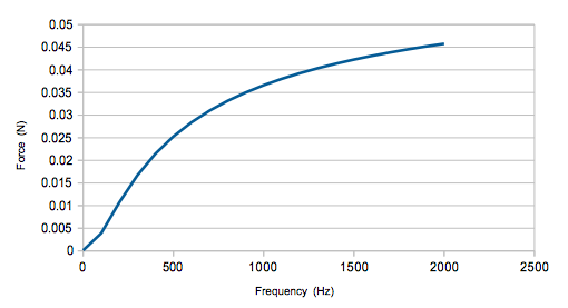
My first order of business was trying to reproduce that plot from Wikipedia that showed the repulsive force going up as frequency went up.
My LUA script opened my FEMM project, saved a temporary copy of it and then started running simulations varying the frequency and measuring force on the coil block. The results were printed to the console:
showconsole()
clearconsole()
mydir="./"
open(mydir .. "pinewood.FEM")
mi_saveas(mydir .. "temp.fem")
print("Frequency","Vertical force (N)")
for n=0,2000,100 do
    mi_deletecircuit("Coil")
    mi_addcircprop("Coil", 3, 1)
    mi_probdef(n,"millimeters","axi",1E-8)
    mi_analyze()
    mi_loadsolution()
    mo_groupselectblock(1)
    fz=mo_blockintegral(12)
    print(n,fz)
end
print("\n")
This console output was easily pasted into a spreadsheet and when graphed produced this:
Hey look, it looks just like the Wikipedia graph!
Playing with FEMM
I was able to determine all kinds of cool stuff with FEMM.
Inductance
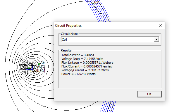
For example, according to this tutorial, in a DC system with only one coil, the measure of magnetic flux per unit current is the inductance of that coil. This is because inductance is also a measure of energy stored in the magnetic field. I deleted the aluminum plate, ran the simulation at 0Hz, and got this:
Or roughly 185
![]()
H. Now how does that compare to Real Life?
In order to calculate the inductance of my real coil, I needed a way to measure how quickly the current changes when I apply a voltage. In order to take this measurement, I place a 0.05
![]()
resistor in series with the coil and measured the voltage across it:
As a sidenote, using an oscilloscope to measure the voltage across a resistor can be a little tricky if you’re feeding it with an AC signal. Oscilloscopes measure voltage relative to a ground reference that you select with the ground clip on the scope probe. The problem is that this ground clip feeds back to Earth ground through the scope itself. If you clip it to one side of the resistor and feed the resistor with an AC signal, you will end up shorting your power supply to ground through your oscilloscope which could damage it!
One way around this is to use an oscilloscope probe on either side of the resistor and connect both of them to a common ground:
There are math functions on most digital scopes that will let you subtract the voltage on one probe from the other. This will give you the voltage across the resistor. The downside of this method is that you have to set the inputs on the scope wide enough to measure two 15V signals. At a 15V range, your precision goes down, so your measurements will be very grainy.
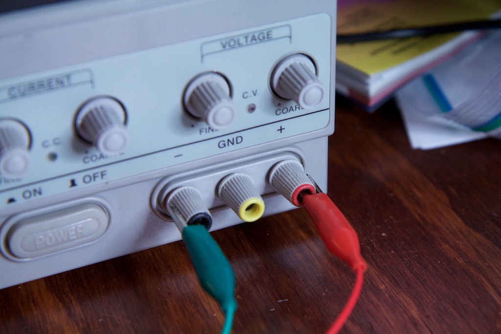
As a better solution, I took advantage of the fact that my power supply has an isolated output:
Connecting to Earth ground is optional, so I don’t have to worry about driving current through the oscilloscope ground clips.
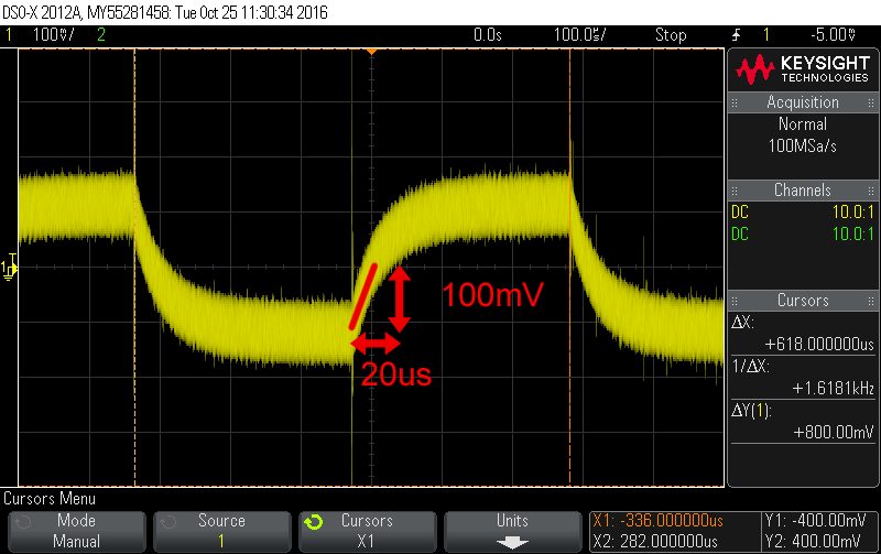
With this config, I could set my scope to 100mV per division and get some quality results.
Here’s a plot I took of the voltage across the 0.05
![]()
resistor in series with my coil which I was driving with a 15V amplitude square wave.
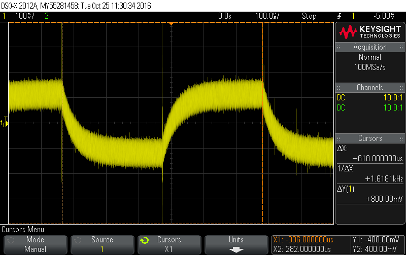 In this plot, the voltage actually represents current since it’s measured across a resistor. each mV corresponds to roughly (
![]()
) 20mA.
So how fast does our current rise?
Roughly 2000mA in 20us. Knowing that we’re driving with 30V (-15V to +15V), what kind of inductance does that give us?
![]()
![]()
![]()
Hey, that’s not bad! 300
![]()
H measured vs 185
![]()
simulated! It could be closer, but it’s also important to note that my real life coil wasn’t perfectly round, and my measurements certainly aren’t super precise. Honestly, I think that it’s a pretty good sign that they’re similar values within the same order of magnitude.
Phase
Remember when I explained how the lag in the aluminum coil current allows the system to repel more than it attracts? I can show that happening in FEMM!
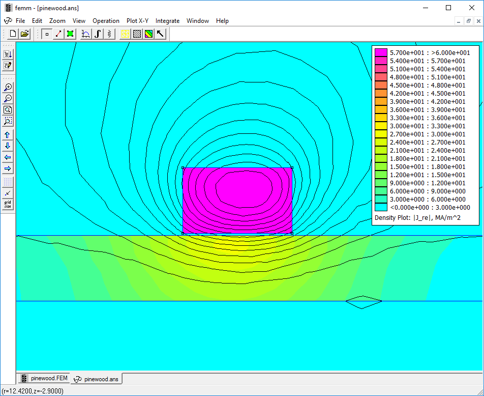
In an oscillatory system like this, many measurements will take on complex values. A complex number is just a way to describe the phase of a measurement. For example, when I want to measure the distribution of current through various parts of my system, I can look at the real current:
You can see that the wire loop is 100% in phase because it’s the current in the loop that’s driving the whole system. It’s in phase with itself.
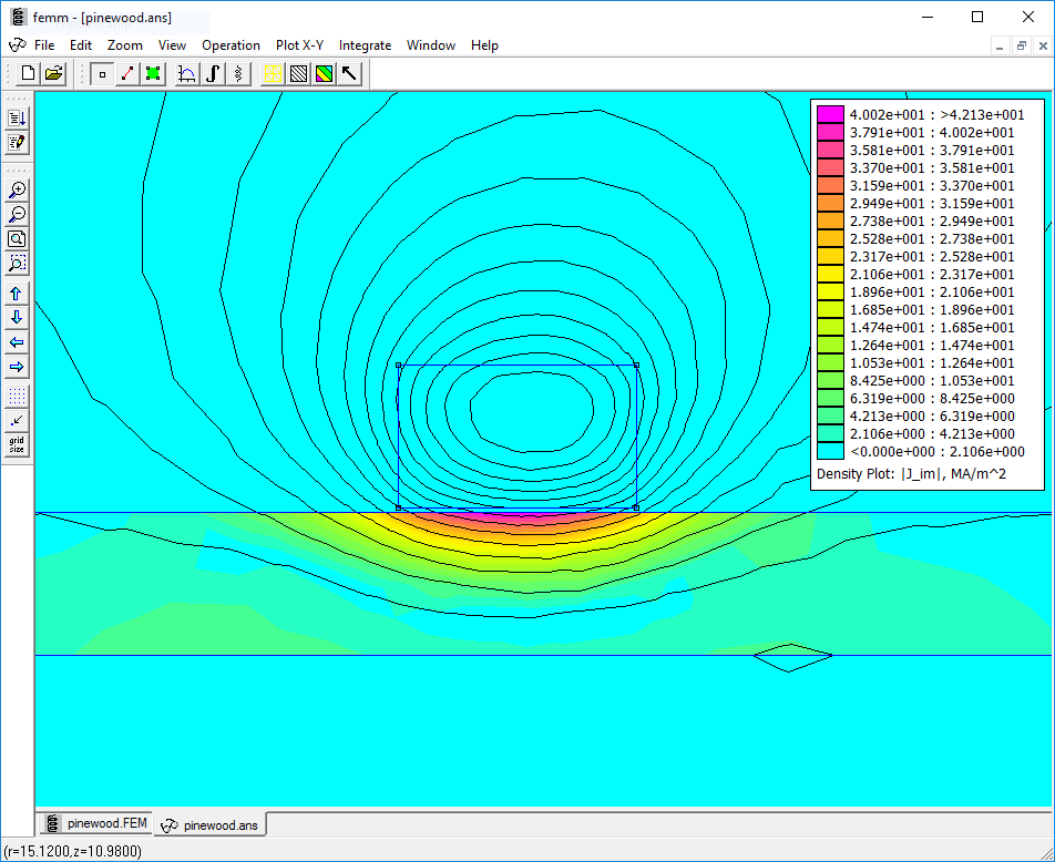
If I look at the imaginary part, I get this:
This describes how out of phase the current is. Obviously my driving coil doesn’t even show up here, but I do get a fair amount of current in the plate right outside the coil.
The real and imaginary parts of a number can be represented on 2D plot where the real part is along the horizontal axis and the imaginary part is on the vertical axis. As a real signal begins to lead or lag on phase, it will become more imaginary. This can be modeled as a rotation of a vector on the real-imaginary plane. Shown below, a purple signal is somewhere between the real signal and 90
![]()
out of phase with that signal. It’s represented with a phase angle
![]()
:
Because my coil levitates best when the driving current and aluminum plate current are 180 degrees out of phase, my target should be to rotate this vector all the way around until it’s facing in the negative direction on the real axis.
I wanted to show how the phase of this current changes with frequency, so I wrote another lua script that measures the current density at a point right below the coil for various frequencies:
print("Frequency","Current Density below coil (MA/m^2)")
for n=0,2000,100 do
    mi_deletecircuit("Coil")
    mi_addcircprop("Coil",3, 1)
    mi_probdef(n,"millimeters","axi",1E-8)
    mi_analyze()
    mi_loadsolution()
    x, x, x, x, x, x, x, Je=mo_getpointvalues(22.5,2.9)
    print(n, Je)
end
And this is what the console spat out:
--> Frequency	Current Density below coil (MA/m^2)
--> 0	0
--> 100	-0.243056486520408-I*1.041375538163957
--> 200	-0.692226764216291-I*1.758839243153171
--> 300	-1.111917985788336-I*2.258829983436955
--> 400	-1.472542570261268-I*2.650430696726264
--> 500	-1.783374971437213-I*2.982991655359612
--> 600	-2.055626083259888-I*3.280740399509312
--> 700	-2.298629570995716-I*3.556590167001452
--> 800	-2.519473644757766-I*3.817664277056517
--> 900	-2.723327352556508-I*4.068052444771565
--> 1000	-2.91393417846034-I*4.310239331611737
--> 1100	-3.094043093791485-I*4.545831712540521
--> 1200	-3.26572057826363-I*4.775927436617781
--> 1300	-3.430559361307798-I*5.001307754101459
--> 1400	-3.589814559888883-I*5.222543338725915
--> 1500	-3.744492977093614-I*5.440057229789597
--> 1600	-3.895413094134038-I*5.654165133594329
--> 1700	-4.043246729999845-I*5.865102941031151
--> 1800	-4.188548984461358-I*6.073046396014496
--> 1900	-4.331780470610597-I*6.278125611115634
--> 2000	-4.473324277664494-I*6.480435989549481
The number formatting is a little gross, so I wrote a quick python script that takes this output as a string and prints out the numbers in polar notation which gives the magnitude and phase angle:
import re
newstring = re.split('\t| |-->|',mystring)
myarray=[]
for i in range(3, len(newstring), 3):
myarray.append(newstring[i])
import cmath
for i in myarray:
print cmath.polar(complex('('+i.replace('I*','')+"j)"))
Here is the result:
(0.0, 0.0)
(1.0693640479864264, -1.8000909698944927)
(1.8901569713526376, -1.9457475384392315)
(2.517672437231139, -2.0282279172160713)
(3.0320231693343853, -2.077918204936272)
(3.475437455154928, -2.109631817676388)
(3.8715444157533447, -2.1305265859093794)
(4.234741021676221, -2.144567154052873)
(4.574090945635257, -2.15413561833756)
(4.895463467598788, -2.160718225979004)
(5.202804579471742, -2.165266484893137)
(5.498880670188968, -2.1684057102776677)
(5.785707716013057, -2.170558502994736)
(6.06480146275968, -2.1720184675944196)
(6.337328104119325, -2.1729947343887566)
(6.604199445723112, -2.1736393768245295)
(6.866136215653219, -2.174064746559392)
(7.123712278618972, -2.174354773192227)
(7.377386740803069, -2.174572566372812)
(7.627527989755882, -2.174765686797981)
(7.874432087953438, -2.1749699018059907)
As you can see, the phase angle quickly shoots to -2.17 radians (about 124
![]()
) and then just stays there. There doesn’t appear to be anything special about this phase angle from a theory point of view. It just falls out of the geometry of the problem. Playing with the thickness of the plate in the simulation will change this angle slightly. This makes sense since measuring the phase angle of eddy currents is actually a method used to identify small cracks or deformities in conductive surfaces such as pipes or fuel tanks.
This does answer a question I had about “tuning” the drive frequency. It looks like you hit the maximum phase angle pretty early and just stay there. This angle depends more on the geometry of the coil than the frequency at which it’s driven.
Table of Contents
The Race and Modeling











Pingback: Fail of the Week: Pinewood Derby Cheat Fails Two Ways | Hackaday
Pingback: Fail of the Week: Pinewood Derby Cheat Fails Two Ways
Pingback: Fail of the Week: Pinewood Derby Cheat Fails Two Ways – Vloda.com
Pingback: Fail of the Week: Pinewood Derby Cheat Fails Two Ways – Celeb Like
Pingback: Fail Of The Week: Pinewood Derby Cheat Fails Two Ways - SLG 2020
drv3h1